CP Scheduler Improvements
Abstract
In July 2014 in APAR VM65288 a customer reported the z/VM Control Program did not enforce relative CPU share settings correctly in a number of scenarios. IBM answered the APAR as fixed-if-next, aka FIN. In z/VM 6.4 IBM addressed the problem by making changes to the z/VM scheduler. The changes solved the problems the customer reported. The changes also repaired a number of other scenarios IBM discovered were failing on previous releases. This article presents an assortment of such scenarios and illustrates the effect of the repairs.
Introduction
In July 2014 in APAR VM65288 a customer reported the z/VM Control Program (CP) did not enforce relative CPU share settings correctly in a number of scenarios. Some of the scenarios were cases in which each guest wanted as much CPU power as CP would let it consume. All CP had to do was to hand out the CPU power in proportion to the share settings. Other scenarios involved what is called excess power distribution, which is what CP must accomplish when some guests want less CPU power than their share settings will let them consume while other guests want more CPU power than their share settings will let them consume. In such scenarios CP must distribute the unconsumed entitlement to the aspiring overconsumers in proportion to their shares with respect to each other.
To solve the problem IBM undertook a study of the operation of the CP scheduler, with focus on how CP maintains the dispatch list. For this article's purposes we can define the dispatch list to be the ordered list of virtual machine definition blocks (VMDBKs) representing the set of virtual CPUs that are ready to be run by CP. The order in which VMDBKs appear on the dispatch list reflects how urgent it is for CP to run the corresponding virtual CPUs so as to distribute CPU power according to share settings. VMDBKs that must run very soon are on the front of the list, while VMDBKs that must endure a wait appear farther down in the list.
The study of how the dispatch list was being maintained revealed CP's algorithms failed to keep the dispatch list in the correct order. One problem found was that CP was never forgetting the virtual CPUs' CPU consumption behavior from long ago; rather, CP kept track of the relationship since logon between the virtual CPU's entitlement to CPU power and its consumption thereof. Another problem found was that the virtual CPUs' entitlements were being calculated over only the set of virtual CPUs present on the dispatch list. As dispatch list membership changed, the entitlements for the members on the dispatch list were not being recalculated and so the VMDBKs' placements in the dispatch list were wrong. Another problem found was that certain heuristics, rather than mathematically justifiable algorithms, were being used to try to adjust or correct VMDBKs' relationships between entitlement and consumption when it seemed the assessment of the relationship was becoming extreme. Another problem found was that the CPU consumption limit for relative limit-shares was not being computed correctly. Still another problem found was that a normalizing algorithm meant to correct entitlement errors caused by changes in dispatch list membership was not having the intended effect.
In its repairs IBM addressed several of the problems it found. The repairs consisted of improvements that could be made without imposing the computational complexity required to keep the dispatch list in exactly the correct order all the time. In this way IBM could improve the behavior of CP without unnecessarily increasing the CPU time CP itself would spend doing scheduling.
Background
In any system consisting of a pool of resource, a resource controller or arbiter, and a number of consumers of said resource, ability to manage the system effectively depends upon there being reliable policy controls whose purpose is to inform the arbiter of how to make compromises when there is more demand for resource than there is resource available to be doled out. For example, when there is a shortage of food, water, or gasoline, rationing rules specify how the controlling authority should hand out those precious commodities to the consumers.
A z/VM system consists of a number of CPUs and a number of users wanting to consume CPU time. The first basic rule for CPU consumption in z/VM is this: for as long as there is enough CPU capacity available to satisfy all users, CP does not restrict, limit, or ration the amount of CPU time the respective users are allowed to consume. The second basic rule for CPU consumption in z/VM is this: when the users want more CPU time than the system has available to distribute, policy expressed in the form of share settings informs CP about how to make compromises so as to ration the CPU time to the users in accordance with the administrator's wishes.
z/VM share settings come in two flavors. The first, absolute share, expresses a user's ration as a percent of the capacity of the system. For example, in a system consisting of eight logical CPUs, a user having an ABSOLUTE 30% share setting should be permitted to run (800 x 0.30) = 240% busy whenever it wants, no matter what the other users' demands for CPU are. In other words, this user should be permitted to consume 2.4 engines' worth of power whenever it desires. The second, relative share, expresses a user's ration relative to other users. For example, if two users have RELATIVE 100 and RELATIVE 200 settings respectively, when the system becomes CPU-constrained and those two users are competing with one another for CPU time, CP must ration CPU power to those users in ratio 1:2.
Share settings are the inputs to the calculation of an important quantity called CPU entitlement. Entitlement expresses the amount of CPU power a user will be permitted to consume whenever it wants. Entitlement is calculated using the system's capacity and the share settings of all the users. Here is a simple example that introduces the principles of the entitlement calculation:
- Suppose the system consists of six logical CPUs, so its capacity is 600%.
- Suppose user UA has a share setting of ABSOLUTE 15%. This share setting means user UA can run (600 x 0.15) = 90% busy whenever it wants.
- The system's promise of 90% to user UA leaves the system with (600-90) = 510% with which to make promises to the other users.
- If we further have users UR1, UR2, and UR3 with
share settings RELATIVE 100, RELATIVE 200, and RELATIVE
300 respectively, those three users' guarantees for,
or entitlements to, CPU power will go like this:
- UR1: 510 x 100/600 = 85%
- UR2: 510 x 200/600 = 170%
- UR3: 510 x 300/600 = 255%
Users' actual CPU consumptions are sometimes below their entitlements. Users who consume below their entitlements leave excess power that can be distributed to users who want to consume more than their entitlements. The principle of excess power distribution says that the power surplus created by underconsuming users should be available to aspiring overconsumers according to their share settings with respect to each other. For example, if we have a RELATIVE 100 and a RELATIVE 200 user competing to run beyond their own entitlements, whatever power the underconsuming users left fallow should be made available to those two overconsumers in a ratio of 1:2.
In addition to letting a system administrator express an entitlement policy, z/VM also lets the administrator specify a limiting policy. By limiting policy we mean z/VM lets the administrator specify a cap, or limit, for the CPU time a user ought to be able to consume, and further, the conditions under which the cap ought to be enforced. The size of the cap can be expressed in either ABSOLUTE or RELATIVE terms; the expression is resolved to a CPU consumption value using the entitlement calculation as illustrated above. The enforcement condition can be either LIMITSOFT or LIMITHARD. The former, LIMITSOFT, expresses that the targeted user is to be held back only to the extent needed to let other users have more power they clearly want. The latter, LIMITHARD, expresses that the targeted user is to be held back no matter what.
The job of the CP scheduler is to run the users in accordance with the capacity of the system, and the users' demands for power, and the entitlements implied by the share settings, and the limits implied by the share settings. In the rest of this article we explore z/VM's behaviors along these lines.
Method
On a production system it can be very difficult to determine whether the scheduler is handing out CPU power according to share settings. The reason is this: the observers do not know the users' demands for CPU power. By demand we mean the amount of CPU power a user would consume if CP were to let the user consume all of the power it wanted. By consumption we mean the amount of CPU power the user actually consumed. Monitor measures consumption; it doesn't measure demand.
To check the CP scheduler for correct behavior it is necessary to run workloads where the users' demands for CPU power are precisely known. To that end, for this project IBM devised a scheduler testing cell consisting of a number of elements.
-
First, IBM built a means, a scripting language of sorts, for
defining a library of scheduler scenarios.
For each such scenario, the scripting language allowed
the definition of all of the following parameters of the
scenario:
- How many logical CPUs (LPUs) are in the LPAR, and what are their types? For example, the LPAR might consist of four CP LPUs, two zIIP LPUs, and three IFL LPUs.
- What is the set of users that will be running during the scenario? For example, users U1, U2, U3, and U4 might all be logged on and competing for CPU time.
- For each such user, what are its share settings for the various LPU types? For example, user U1 might have a relative 100 share on CPs, a relative 200 share on IFLs, and an absolute 30% share on zIIPs.
- For each such user, what virtual CPUs are defined for it? For example, user U1 might have a virtual CP at virtual CPU address 0 and a virtual IFL at virtual CPU address 1.
- For each such virtual CPU, what is its demand for CPU power? For example, for U1's virtual CPU 2, the virtual CPU might run to 35% busy if it could get all of the CPU power it wanted.
-
Next, IBM built a number
of scenarios for the scenario library.
The scenarios were devised
to exercise CP in a number of different
ways, for example:
- The scenarios reported in VM65288
- Scenarios in which every virtual CPU in the scenario wanted to consume as much CPU power as CP would allow, so CP ought to distribute the CPU power according to the share settings
- Scenarios in which some virtual CPUs wanted less CPU power than their share settings would permit, while other virtual CPUs wanted more, so to solve the scenario CP would have to implement excess power distribution correctly
- Scenarios that mixed relative-share users and absolute-share users
- Scenarios that exercised LIMITSOFT
- Scenarios that exercised LIMITHARD
-
Next, IBM built software that would
read a scenario definition and
calculate mathematically what the virtual CPUs'
CPU utilizations would be
if CP were to
behave exactly correctly. This program, called the solver,
used the mathematics behind the problem of excess power distribution
to do the computation.
-
Next, IBM built a CPU burner program
that could run in a virtual N-way
guest. The burner's command line would accept a description of
the virtual CPUs of the guest and the CPU utilization target it
should
try to achieve on each virtual CPU. For example, if
the guest were a virtual 2-way with one virtual CP and one
virtual IFL, the burner could be told to try to run the virtual
CP 65% busy and the virtual IFL 81% busy.
On each virtual CPU,
to achieve the utilization target
the burner used a combination of
a spin loop, plus
calls to Diag x'0C', plus
the clock comparator.
-
Next, IBM built software that would
read a scenario definition and
instantiate the problem on an LPAR:
configure the LPAR with the correct numbers and types of logical CPUs,
log on all of the scenario's users,
define for each user its prescribed virtual CPUs,
issue for each user its prescribed CP SET SHARE commands, and
set each user in motion running the CPU burner according to
the CPU utilization targets specified for the user's
virtual CPUs.
This program, called the runner,
also included job steps
to start and stop MONWRITE, and
to run Perfkit to reduce the MONWRITE file, and
to mine the Perfkit listing so
as to extract the actual CPU consumptions of the virtual CPUs
comprising the scenario.
-
Last, IBM built software
for comparing the correct answers
calculated by the solver to
the observed behaviors produced
by the runner.
This program, called the comparator,
was able to form a scalar expression of the error CP
committed during the running of the scenario.
The scalar error
was calculated by treating
the solver's correct answer and
the runner's observed result
each as an N-dimensional vector,
where each dimension expressed the CPU consumption of one of
the N virtual CPUs of the measurement.
The N-dimensional vector drawn
from the tip of the correct result's vector
to the tip of the
observed result's vector,
called the error vector, represents the error CP
committed in the running of the scenario.
The CP error was then quantified
as the
magnitude of the error vector divided by the magnitude
of the correct answer vector.
The magnitudes of the correct answer vector
and the error vector
were calculated
using the Cartesian
distance formula for N dimensions.
Figure 1 illustrates the error calculation for an experiment using two virtual CPUs. The correct utilizations and observed utilizations appear in the table on the left of the figure. The correct answer vector and the error vector are illustrated in the graph on the right. The run error is calculated as the magnitude of the error vector divided by the magnitude of the correct answer vector. The error is then converted to a percent by multiplying by 100. When the scenario uses more than two virtual CPUs, it becomes difficult to plot the vectors but the calculation proceeds in the same way.
Figure 1. Calculating scheduler error. 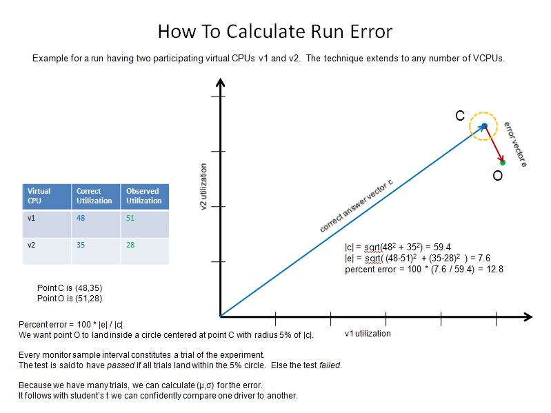
Results and Discussion
The scenario library used was too large for this report to illustrate every case. Rather for this report we have chosen an assortment of scenarios so as to illustrate results from a variety of configurations.
Infinite Demand, Equal Share
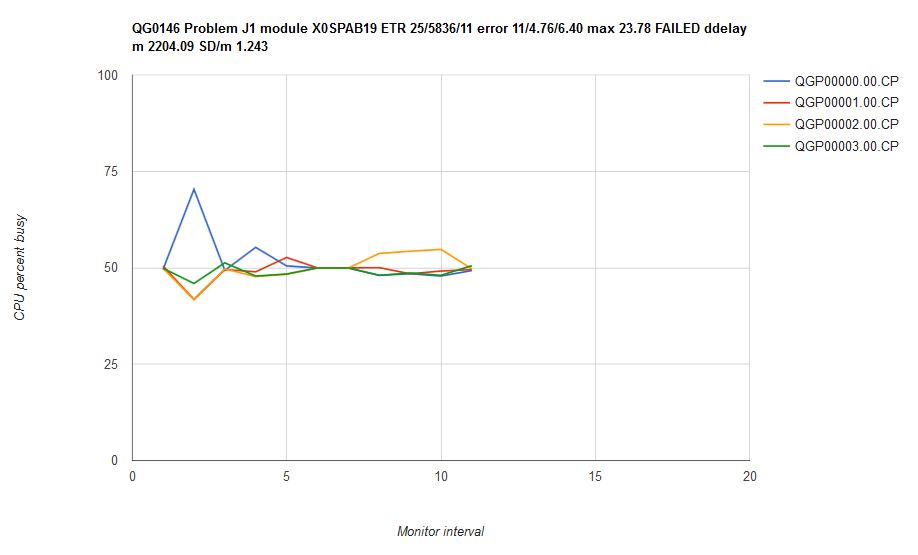
Figure 2 illustrates the scenario for the simplest problem reported in VM65288. In this scenario, which we called J1, each virtual CPU wants as much power as CP will let it consume. All CP has to do is distribute power according to the share settings. Further, the share settings are equal to one another, so all virtual CPUs should run equally busy.
| Figure 2. Scenario J1 from VM65288. Two logical CPs, four virtual uniprocessor guests, all virtual CPUs wanting infinite power, and all guests having relative 100 share on CPs. |
|
|
In such a scenario each of the four virtual CPUs should run (200/4) = 50% busy constantly. However, that is not what happened. Figure 3 illustrates the result of running scenario J1 on z/VM 6.3. The graph portrays CPU utilization as a function of time for each of the four virtual CPUs of the measurement: QGP00000.0, QGP00001.0, QGP00002.0, and QGP00003.0. The four users' CPU consumptions are not steady, and further, virtual CPU QGP00000.0 shows an excursion near the beginning of the measurement. Mean CP error was 4.76% with a max error of 23.78%. We classified this result as a failure.
| Figure 3. Scenario J1 run on z/VM 6.3 with all service closed as of November 19, 2015. Machine type is z13. |
|
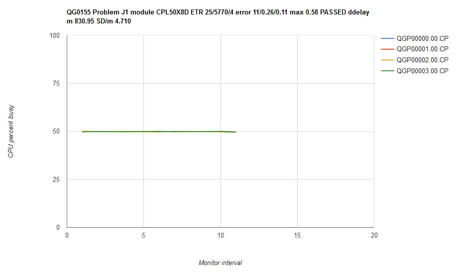
Figure 4 illustrates what happened when we ran scenario J1 on an internal CP driver containing the scheduler fixes. Each of the four virtual CPUs runs with 50% utilization, and further, the utilizations are all constant over time. Mean CP error was 0.26% with a max error of 0.58%. We classified this result as a success.
| Figure 4. Scenario J1 run on internal driver CPL50X8D which contains the scheduler repairs. Machine type is z13. |
|
A side effect of repairing the scheduler was that the virtual CPUs' dispatch delay (on the chart title, ddelay) experience improved. In the z/VM 6.3 measurement above, virtual CPUs ready to run experienced a mean delay of 2204 microseconds between the instant they became ready for dispatch and the instant CP dispatched them. In the measurement on the internal driver, mean dispatch delay dropped to 831 microseconds. The dispatch delay measurement came from monitor fields the March 2015 SPEs added to D4 R3 MRUSEACT.
Infinite Demand, Unequal Share
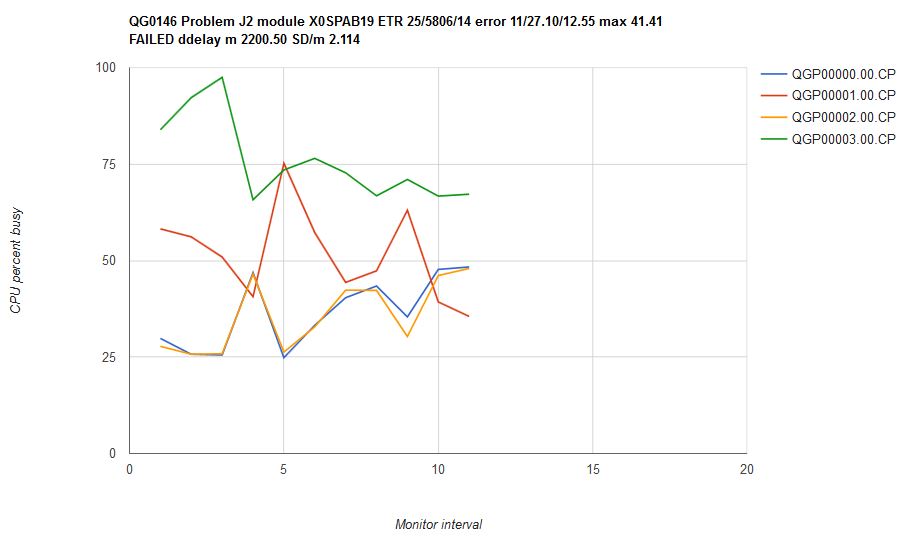
Figure 5 illustrates the scenario for another problem reported in VM65288. In this scenario, which we called J2, each virtual CPU wants as much power as CP will let it consume. All CP has to do is distribute power according to the share settings. Unlike J1, though, the share settings are unequal. In this case CP should distribute CPU power in proportion to the share settings.
| Figure 5. Scenario J2 from VM65288. Two logical CPs, four virtual uniprocessor guests, all virtual CPUs wanting infinite power, and the guests having unequal relative share settings. |
|
|
In such a scenario the four virtual CPUs should run with CPU utilizations in ratio of 1:2:1:4, just as their share settings are. However, that is not what happened. Figure 6 illustrates the result of running scenario J2 on z/VM 6.3. The four users' CPU consumptions are not steady, and further, the consumptions are out of proportion. Mean CP error was 27.1% with a max error of 41.4%. We classified this result as a failure.
| Figure 6. Scenario J2 run on z/VM 6.3 with all service closed as of November 19, 2015. Machine type is z13. |
|
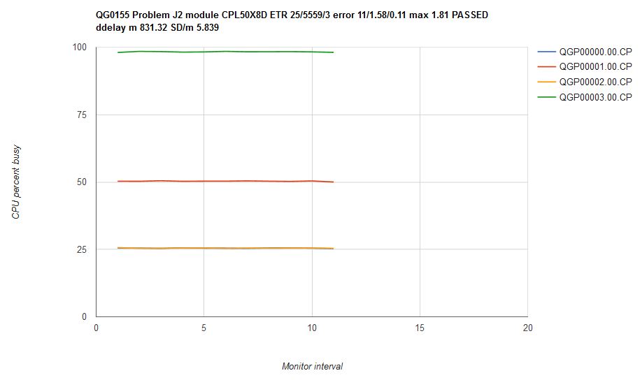
Figure 7 illustrates what happened when we ran scenario J2 on an internal CP driver containing the scheduler fixes. The CPU consumptions are steady over time and are in correct proportion. Mean CP error was 1.58% with a max error of 1.81%. We classified this result as a success.
| Figure 7. Scenario J2 run on internal driver CPL50X8D which contains the scheduler repairs. Machine type is z13. |
|
Donors and Recipients, Unequal Shares
Figure 8 illustrates a scenario inspired by what we saw reported in VM65288. In this scenario, which we called J3, some virtual CPUs, called donors, require less CPU time than their entitlements assure them. Further, other virtual CPUs, called recipients, have infinite demand. To behave correctly CP must distribute the donor users' unconsumed entitlement to the aspiring overconsumers in proportion to their share settings with respect to each other. In other words, CP must correctly implement the principle of excess power distribution.
| Figure 8. Scenario J3 inspired by VM65288. Two logical CPs, six virtual uniprocessor guests, some virtual CPUs wanting infinite power, and other virtual CPUs wanting less power than that to which they are entitled. Share settings vary. |
|
|
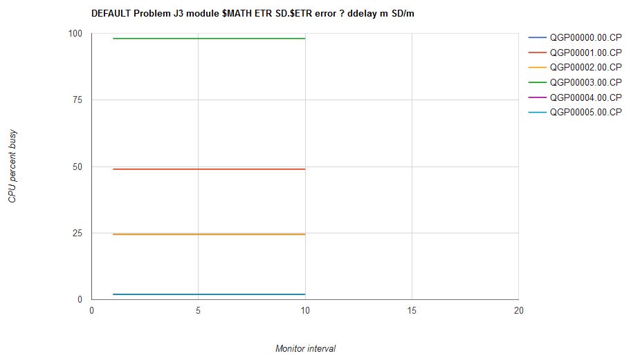
Unlike in the previous scenarios, the correct answer for scenario J3 isn't easily computed mentally. This is where we made use of the solver. Figure 9 illustrates the solver's output for scenario J3. The solver implements the mathematics of excess power distribution to calculate what CP's behavior ought to be.
| Figure 9. Scenario J3 solution computed by the solver. |
|
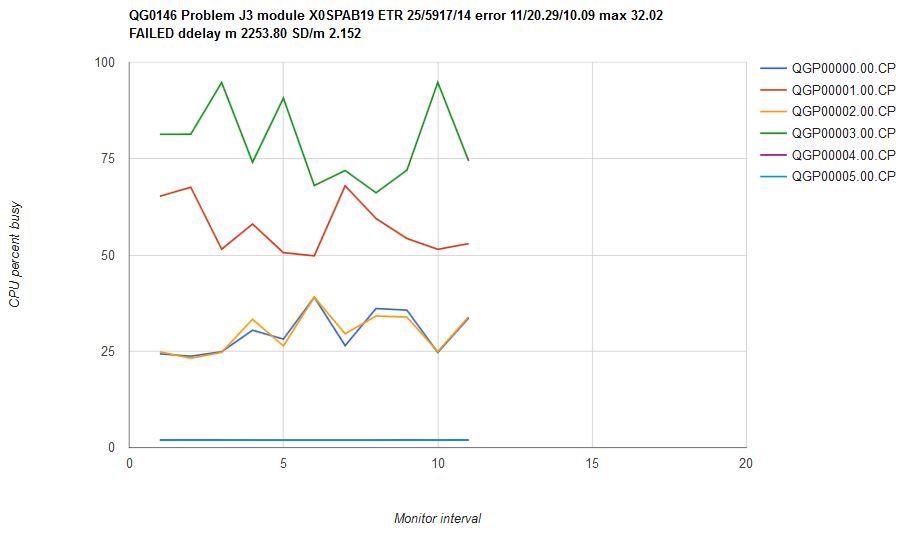
Figure 10 illustrates what happened when we ran scenario J3 on z/VM 6.3. The CPU consumptions are unsteady over time and are not in correct proportion. Mean CP error was 20.29% with a max error of 32.02%. We classified this result as a failure.
| Figure 10. Scenario J3 run on z/VM 6.3 with all service closed as of November 19, 2015. Machine type is z13. |
|
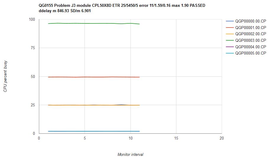
Figure 11 illustrates what happened when we ran scenario J3 on an internal CP driver containing the scheduler fixes. The CPU consumptions are steady over time and are in correct proportion. Mean CP error was 1.59% with a max error of 1.90%. We classified this result as a success.
| Figure 11. Scenario J3 run on internal driver CPL50X8D which contains the scheduler repairs. Machine type is z13. |
|
More Donors, More Recipients, and Unequal Shares
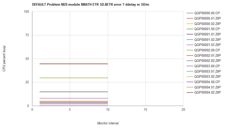
Figure 12 illustrates scenario MZ0 that is a more complex variant of scenario J3. Here there are more donors and more recipients. Also, the scenario runs on the zIIPs of a mixed-engine LPAR. Again, to run this scenario CP must correctly implement the principle of excess power distribution.
| Figure 12. Scenario MZ0. |
|
|
As was true for J3, to see the correct answer for MZ0 we need to use the solver. Figure 13 illustrates the solver's output for scenario MZ0.
| Figure 13. Scenario MZ0 solution computed by the solver. |
|
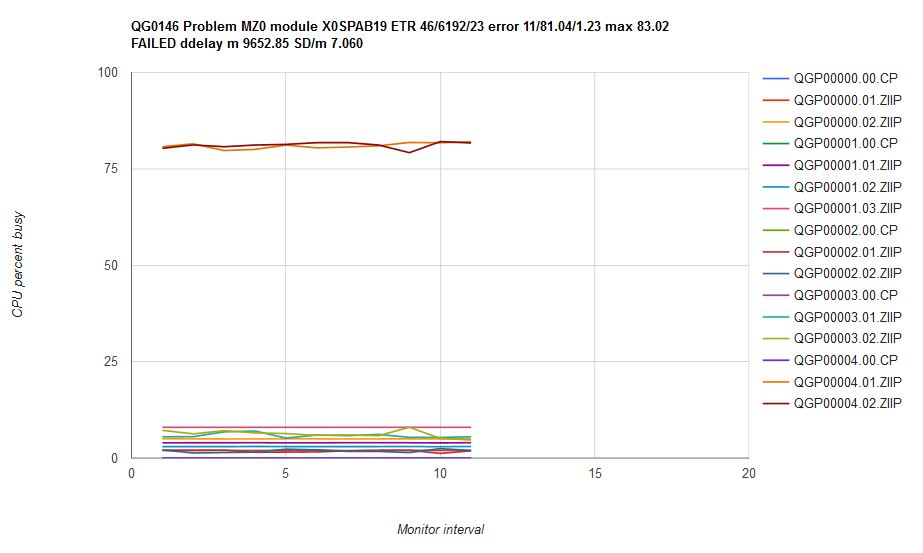
Figure 14 illustrates what happened when we ran scenario MZ0 on z/VM 6.3. The CPU consumptions are fairly steady over time, but they are not in correct proportion. The high-entitlement users got a disproportionately large share of the excess. Mean CP error was 81.04% with a max error of 83.02%. We classified this result as a failure.
| Figure 14. Scenario MZ0 run on z/VM 6.3 with all service closed as of November 19, 2015. Machine type is z13. |
|
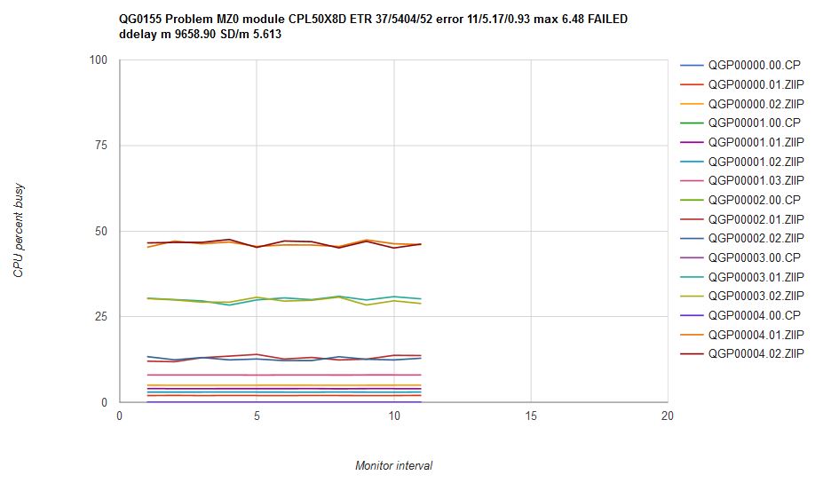
Figure 15 illustrates what happened when we ran scenario MZ0 on an internal CP driver containing the scheduler fixes. The CPU consumptions are fairly steady over time and are in about the correct proportion. Mean CP error was 5.17% with a max error of 6.48%. Our comparator printed "FAILED" on the graph, but given how much better the result was, we felt this was a success.
| Figure 15. Scenario MZ0 run on internal driver CPL50X8D which contains the scheduler repairs. Machine type is z13. |
|
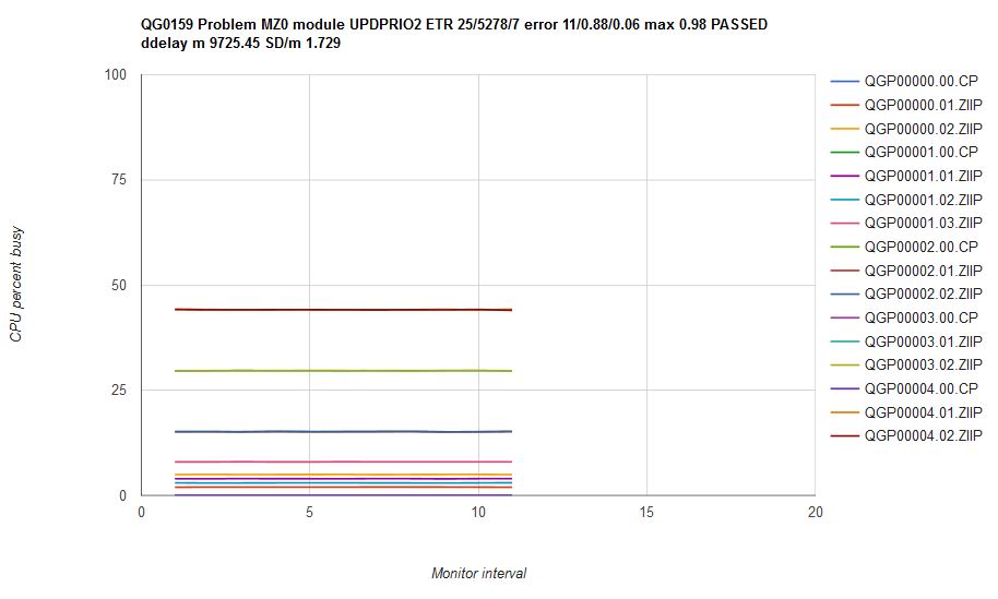
In studying the cause of the vibration in scenario MZ0 we decided to write an additional repair for the CP scheduler. We wrote a mathematically correct but potentially CPU-intensive modification we were certain would improve dispatch list orderings. We then ran scenario MZ0 on that experimental CP. Figure 16 illustrates what happened in that run. The CPU consumptions are steady and in correct proportion. Mean CP error was 0.88% with a max error of 0.98%. In other words, this experimental CP produced correct results. However, we were concerned the modification we wrote would not scale to systems housing hundreds to thousands of users, so we did not include this particular fix in z/VM 6.4.
| Figure 16. Scenario MZ0 run on internal driver UPDPRIO2 which contains the experimental scheduler repair. Machine type is z13. |
|
ABSOLUTE LIMITHARD, With a Twist
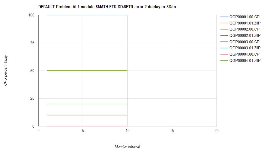
Figure 17 illustrates scenario AL1 which we wrote to check ABSOLUTE LIMITHARD. Here there are donors, recipients, and a LIMITHARD user. To run this scenario CP must hold back the LIMITHARD user to its limit and must correctly implement the principle of excess power distribution.
| Figure 17. Scenario AL1. |
|
|
The apparently correct answer for scenario AL1 is calculated like this:
- The LPAR has two logical zIIPs aka 200% capacity
- QGP00004.0 will run (200 x 0.25) = 50% busy
- This leaves (200-50) = 150% for the other three users
- QGP00001 and QGP00002 will consume (10+20) = 30%
- This leaves (150-30) = 120% for QGP00003 if it wants it
- But QGP00003 has only one virtual zIIP
- Therefore QGP00003 ought to run 100% busy
The solver found the above solution too. Figure 18 illustrates the solver's output for scenario AL1.
| Figure 18. Scenario AL1 solution computed by the solver. |
|
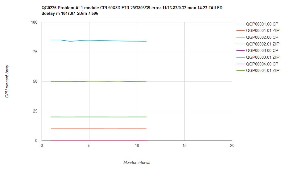
Figure 19 illustrates what happened when we ran scenario AL1 on an internal CP driver containing the scheduler fixes. The CPU consumptions are steady over time. Further, the two donor users and the ABSOLUTE LIMITHARD user all have correct CPU consumptions. It seems, though, there is a problem with the unlimited user. The solver calculated QGP00003 should have run 100% busy but it did not. Thus the comparator classified the run as a failure.
| Figure 19. Scenario AL1 run on internal driver CPL50X8D which contains the scheduler repairs. Machine type is z13. |
|
It took a while for us to figure out that the problem here was not that CP had run scenario AL1 incorrectly. In fact, CP had run the scenario exactly correctly; rather, it was the solver that was wrong. A basic assumption in the solver's math is that if there is more CPU power left to give away, and if there is a user who wants it, CP will inevitably give said power to said user. As we studied the result we saw said assumption is false. When there are only a few logical CPUs to use and the CPU consumptions of the virtual CPUs are fairly high, it is not necessarily true that CP will be able to give out every last morsel of CPU power to virtual CPUs wanting it. Rather, some of the CPU capacity of the LPAR will unavoidably go unused. The situation is akin to trying to put large rocks into a jar that is the size of two or three such rocks. Just because there is a little air space left in the jar does not mean one will be able to fit another large rock into the jar. The leftover jar space, the gaps between the large rocks, is unusable, even if the volume of the leftover space exceeds the volume of the desired additional rock. The same is true of the capacity of the logical CPUs in scenario AL1.
The proof of the large jar hypothesis for scenario AL1 lies in a probabilistic argument. Here is how the proof goes.
- The probabilities of the two donors and the LIMITHARD
user occupying logical CPUs are exactly their observed
CPU utilizations:
- QGP00001: p=0.10 (10% busy)
- QGP00002: p=0.20 (20% busy)
- QGP00004: p=0.50 (50% busy)
- If CP is behaving correctly, the probability that unlimited user QGP00003 is occupying a logical CPU ought to be exactly equal to the probability that CP has a logical CPU available to run it.
-
The probability that CP has a logical CPU available to run
QGP00003 is equal to 1 minus the sum of the probabilities
of the occupancy scenarios that prevent QGP00003 from running:
- QGP00001 and QGP00002: (0.10 x 0.20) = 0.02
- QGP00001 and QGP00004: (0.10 x 0.50) = 0.05
- QGP00002 and QGP00004: (0.20 x 0.50) = 0.10
- Sum = (0.10 + 0.05 + 0.02) = 0.17
- Occupancy opportunity for QGP00003 = 1 - 0.17 = 0.83
- Therefore QGP00003 ought to run 83% busy.
Some readers might notice that if the system administrator had used the CP DEDICATE command to dedicate a logical CPU to user QGP00003, CP might have satisifed all users, like so:
- QGP00003 dedicated onto logical CPU 1: 100% busy
- Users QGP00001, QGP00002, and QGP00004 sharing logical CPU 0: (10% + 20% + 50%) = 80% busy
There is an old maxim floating around the performance community. The saying goes, "When the system is not completely busy, every user must be getting all the CPU power he wants." Scenario AL1 teaches us the maxim is false. This lesson helps us to understand why in a Perfkit USTAT or USTATLOG report we might see %CPU samples even though the system is not completely busy, or why in a Perfkit PRCLOG report we might see logical CPU %Susp even though it appears the CPC has more power to give.
Notes on ETR
The CPU burner program prints a transaction rate that is proportional to the number of spin loops it accomplishes. The system's overall ETR is taken to be the sum of the users' individual transaction rates. Each of the graph titles above expresses the run's ETR in the form n/m/sd, where n is the number of samples of ETR we collected, m is the mean of the samples of ETR, and sd is the standard deviation of the samples of ETR. Readers will notice that we sometimes saw an ETR drop in z/VM 6.4 compared to z/VM 6.3. This must not be taken to be a failure of z/VM 6.4. Rather, it is inevitable that ETR will change because z/VM has changed how it distributes CPU power to the users comprising the measurement.
Notes on Dispatch Delay
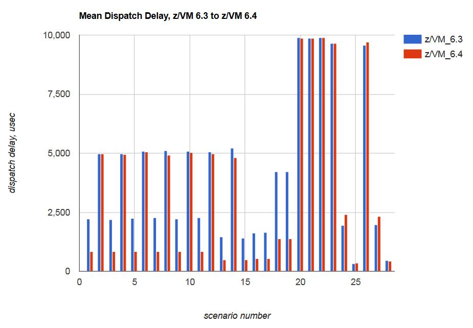
In discussing the results for scenario J1 we mentioned that on z/VM 6.4 the virtual CPUs experienced reduced mean dispatch delay compared to z/VM 6.3. In surveying the results from the whole scenario library we found several scenarios experienced reduced mean delay. Figure 20 illustrates the scenarios' dispatch delay experience. Decreasing mean dispatch delay was not one of the project's formal objectives but the result was nonetheless welcome.
| Figure 20. Mean dispatch delay, z/VM 6.3 to z/VM 6.4. |
|
Remaining Problem Areas
Our scenario library included test cases that exercised share setting combinations we feel are less commonly used. We included a LIMITSOFT case and a RELATIVE LIMITHARD case. Our tests showed LIMITSOFT and RELATIVE LIMITHARD still need work.
LIMITSOFT
By LIMITSOFT we mean a consumption limit CP should enforce only when doing so lets some other user have more power. Another way to say this is that provided it wants the power, a LIMITSOFT user gets to have all of the power that remains after:
- All unlimited users consume all of the power they want, and
- All LIMITHARD users consume either their limit or all the power they want, whichever is less.
Figure 21 illustrates scenario SL3 that employs LIMITSOFT. The scenario runs on a single logical zIIP. There are three virtual CPUs: one donor, one unconstrained recipient, and one ABSOLUTE LIMITSOFT recipient.
| Figure 21. Scenario SL3, a LIMITSOFT scenario. |
|
|
We can calculate the correct answer for SL3. Here is how the calculation goes.
- The capacity of the LPAR is 100%.
- The users' entitlements are calculated using their min-shares.
- All users' min-shares are the same, RELATIVE 100.
- Therefore each user has entitlement (100/3) = 33% busy.
- Therefore donor QGP00001 will run 2% busy.
- The limit-share for user QGP00004 is ABSOLUTE 10% or (100 x 0.10) = 10% busy. Yes, this is less than its min-share entitlement of 33%, but the limit-share still governs.
- The system has 98% busy left to distribute between the unconstrained recipient and the ABSOLUTE LIMITSOFT user.
- The LIMITSOFT user QGP00004 will be held to 10% busy.
- The unconstrained recipient QGP00003 will run 88% busy.
The solver agrees. Figure 22 illustrates the solver's output for scenario SL3.
| Figure 22. Scenario SL3 solution computed by the solver. |
|
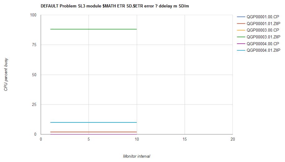
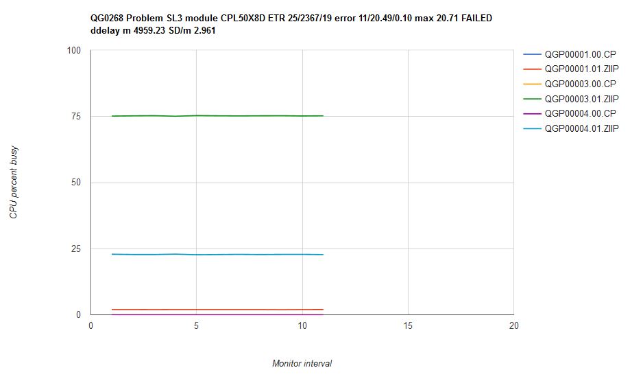
Figure 23 illustrates what happened when we ran scenario SL3 on an internal driver that contained the scheduler repairs.
| Figure 23. Scenario SL3 run on internal driver CPL50X8D which contains the scheduler repairs. Machine type is z13. |
|
The LIMITSOFT user was not held back enough, and the unconstrained recipient did not get enough power.
RELATIVE LIMITHARD
Like ABSOLUTE LIMITHARD, RELATIVE LIMITHARD expresses a hard limit on CPU consumption. The difference is that the CPU consumption cap is expressed in relative-share notation rather than as a percent of the capacity of the system. As part of our work on this project we ran a simple RELATIVE LIMITHARD test to see whether CP would enforce the limit correctly.
Figure 24 illustrates scenario MR2 that employs RELATIVE LIMITHARD. The scenario runs on the logical zIIPs. There are two virtual CPUs: one that runs unconstrained and one that ought to be held back.
| Figure 24. Scenario MR2, a RELATIVE LIMITHARD scenario. |
|
|
The correct answer for scenario MR2 is calculated like this:
- The LPAR's capacity is 200%
- The sum of the relative shares relevant in the calculation of the limit for user QGP00001 is (200+50) = 250
- User QGP00001 should be limited to (200 x 50/250) = 40% busy
- The system has (200-40) = 160 capacity remaining
- User QGP00000 has only one virtual zIIP
- Therefore user QGP00000 should run 100% busy
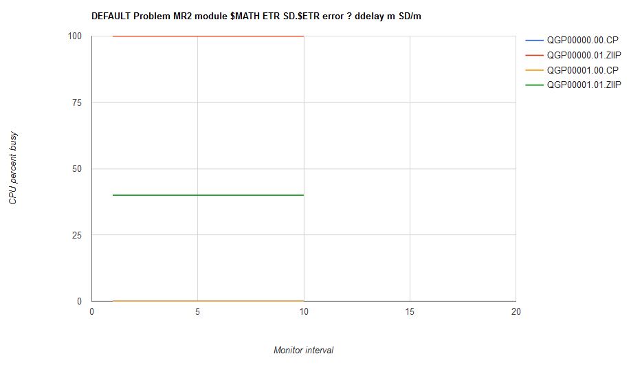
Figure 25 shows us the solver produced the same answer:
| Figure 25. Scenario MR2 solution computed by the solver. |
|
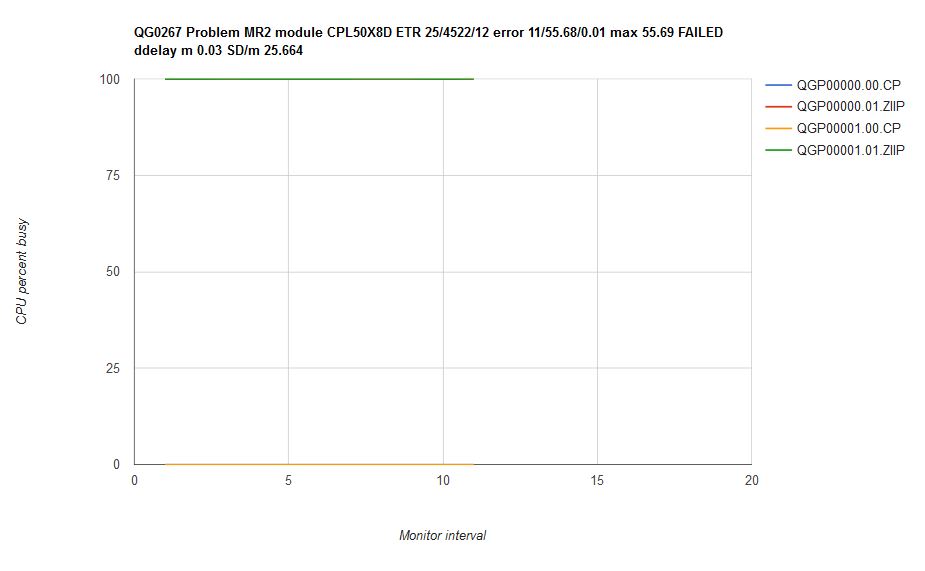
Figure 26 illustrates what happened when we ran scenario MR2 on an internal driver that contained the scheduler repairs.
| Figure 26. Scenario MR2 run on internal driver CPL50X8D which contains the scheduler repairs. Machine type is z13. |
|
CP did not enforce the RELATIVE LIMITHARD limit, rather, it let user QGP00001's virtual zIIP run unconstrained.
Let's return to the hand calculation of the CPU consumption limit for scenario MR2's RELATIVE LIMITHARD user. When a user's limit-share is expressed with relative-share syntax, the procedure for calculating the CPU consumption limit is this:
- Form the set of min-share settings of all the guests. Call this set S.
- Remove from S the min-share setting for the RELATIVE LIMITHARD user.
- Add to S the limit-share setting for the RELATIVE LIMITHARD user.
- Using the adjusted set S and the usual procedure for calculating entitlement, calculate the entitlement for the RELATIVE LIMITHARD user.
- The result of the entitlement calculation is the CPU consumption limit for the RELATIVE LIMITHARD user.
For a couple of reasons, we question whether relative limit-share has any practical value as a policy knob. One reason is the complexity of the above calculation increases as the number of logged-on users increases. Another reason is that as users log on, log off, or incur changes in their share settings, the CPU consumption cap associated with the relative limit-share will change. For these reasons we feel on a large system it would be quite difficult to predict or plan the CPU utilization limit for a user whose limit-share were specified as relative. Overcoming this would require a tool such as this study's solver and would require the system administrator to run it each time his system incurred a logon, a logoff, or a CP SET SHARE command.
Mixing Share Flavors for a Single Guest
In a recent PMR IBM helped a customer to understand what was happening to a guest for which he had specified the share setting like this:
- Base case: SHARE ABSOLUTE 25%
- Comparison case: SHARE ABSOLUTE 25% RELATIVE 200 LIMITHARD
In the base case, the user consumed more than 25% of the system's capacity. In the comparison case, the user, whose demand had not changed, was being held back to less than 25% of the system's capacity.
Here is what happened. Owing to the share settings of the users on the customer's system, the limit-share setting, RELATIVE 200 LIMITHARD, calculated out to be a more restrictive policy than the min-share setting of ABSOLUTE 25%. The customer's mental model for what the command does -- which, by the way, was probably abetted by IBM's use of the phrases minimum share and maximum share in its description of the command syntax -- was that the limit-share clause of the SET SHARE command specifies a more permissive value than does the min-share clause of the command. Even though IBM calls those tokens minimum share and maximum share, the math will sometimes work out otherwise. The lesson here is to be very careful in mixing share flavors within the settings of a single guest.
Summary and Conclusions
Observing whether the scheduler is behaving correctly is very difficult on a production system. Therefore checking the scheduler requires the building of a measurement cell where all factors can be controlled.
In the scenarios of VM65288, and in several others IBM tried, z/VM 6.4 enforces share settings with less error than z/VM 6.3 did. A side effect was that dispatch delay was reduced in many of the scenarios.
The LIMITSOFT and RELATIVE LIMITHARD limiting features might fail to produce intended results in some situations.
The effect of a relative limit-share setting might be difficult to predict or to plan. Thus the practical value of relative limit-share as a policy tool is questionable.
Mixing share flavors on a single guest requires careful thought.