Eighty Logical Processors
Abstract
New function Eighty Logical Processors increases the processor support limit on the z14 from 64 logical processors to 80 logical processors. To check scalability we ran sets of runs using a memory-rich Linux AWM-Apache workload and sets of runs using a memory-constrained Linux AWM-Apache workload. We found most measurements scaled correctly. Customers aspiring to run large partitions with a substantial number of guests all coupled to a single layer-3 vswitch will want to proceed with caution. We did not find any other scaling problems up through 80 processors.
PTF UM35474 for APAR VM66265 implements the new function.
Customer results will vary according to system configuration and workload.
Background
New function Eighty Logical Processors increases the processor support limit from 64 logical processors to 80 logical processors. The increase is for only the z14. The increased limit recognizes some customers' desire to run partitions larger than the previous support limit.
More specifically, the support limit works like this: the largest processor number (sometimes called "processor address") supported in a z/VM partition is now x'4F', aka decimal 79. Because the selections made for partition mode, processor types, and SMT setting affect how processors are numbered, the actual number of processors present in a partition whose largest processor number is x'4F' will vary. Table 1 illustrates how the limit plays out, according to the partition mode, and the types of cores present in the partition, and the SMT setting.
| Table 1. Partition configurations and limits. | |||
|
Partition in Linux-only mode |
|||
| Core types | Non-SMT | SMT-1 | SMT-2 |
| All CPs |
|
|
|
| All IFLs |
|
|
|
|
Partition in z/VM mode |
|||
| Core types | Non-SMT | SMT-1 | SMT-2 |
| Mixed CPs and other types |
|
|
|
|
Partition in any other supported mode |
|||
| Core types | Non-SMT | SMT-1 | SMT-2 |
| Any supported configuration |
|
|
|
Claiming z/VM supports a certain number of logical processors requires far more than just setting array sizes, bit mask lengths, and other constants so all those processors can be handled in a functionally correct way. Rather, to decide whether we can claim to support n logical processors, we run workloads to check whether the system's performance exhibits what we call correct scaling. By this we mean for selected workloads the partition gains capacity in correct proportion to the number of processors added. Now, we cannot check scaling on every possible workload, nor is it necessary for z/VM to exhibit correct scaling on every conceivable workload. Rather, we check scaling on workloads we feel would show us whether some kind of pervasive software scaling problem exists in the z/VM Control Program.
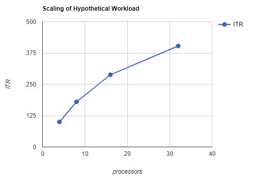
By check scaling we mean we run a given workload in larger and larger configurations in larger and larger partitions and look at how the system performs as we scale up. For example, we might make up a workload that can be run in a variety of sizes by varying the number of participating guests. We might then run the 16-guest edition in a 4-processor partition, and the 32-guest edition in an 8-processor partition, and so on. We would record ITR for each run and then graph ITR as a function of partition size. This procedure gives us a scaling curve that shows how this workload scales as we add both burden and resource. Figure 1 shows the scaling behavior of a hypothetical workload.
| Figure 1. Scaling of hypothetical workload. |
|
| Notes: This hypothetical data illustrates the general shape of a scaling curve. |
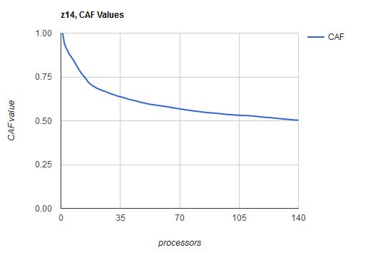
The Z Systems CPC itself gives us information that helps us decide whether we are observing correct scaling. As part of developing each Z Systems processor family, IBM Z Systems Processor Development runs a suite of reference workloads built in such a way that the workloads themselves contain no barriers to scaling. Those workloads are run in increasing sizes in partitions of increasing numbers of processors. All runs are memory-rich and non-SMT. Each run is done in such a way that the partition's average logical processor is about 90% busy (FCX225 SYSSUMLG). The results are tallied and then converted into an array of scalars called Capability Adjustment Factors or CAF values. For a partition of n processors we derive a corresponding CAF value cn, 0<cn<=1. The value cn represents how much effective capability each of the n processors brings to the partition. Of course, for a partition of one processor, c1=1. On the z14, for a partition of two processors, c2=0.941; this means the two-processor partition has an effective capability of (2 x 0.941) or 1.882 units of capability. The instruction Store System Information (STSI) returns the CAF values. Figure 2 shows a plot of z14 CAF values as a function of number of processors. Remember these CAF values were derived from the behavior of IBM's reference workloads.
| Figure 2. z14 CAF values. |
|
| Notes: 3906-M05 s/n E46E7, 2019-03-30. Physical cores: 4 CPs, 4 ICFs, 4 zIIPs, 128 IFLs. |
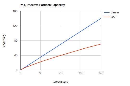
As intimated above, the capability of a partition of n processors is (n x cn). Figure 3 plots the effective partition capability for a z14 as assessed by IBM's reference workloads. For illumination, on the same graph we plotted linear scaling.
| Figure 3. z14 effective partition capability. |
|
| Notes: Effective capability EC(n) = n x cn. |
To compute how the capability of an m-processor partition compares to the capability of an n-processor partition, we just calculate the ratio (m x cm) / (n x cn). Using this technique we can draw an expectation curve for how, for example, the capabilities of 32-processor, 48-processor, and 64-processor partitions compare to the capability of a 16-processor partition. Table 2 illustrates how this is done. We'll use such curves later, in the results section of this chapter.
| Table 2. Comparing partition capabilities. | |||||
| Processors | 16 | 32 | 48 | 64 | 80 |
| CAF value cn | 0.721 | 0.646 | 0.603 | 0.578 | 0.554 |
| Capability n x cn | 11.54 | 20.67 | 28.94 | 36.99 | 44.32 |
| Capability ratio | 1.00 | 1.79 | 2.51 | 3.21 | 3.84 |
| Notes: 3906-M05 s/n E4E67, 2019-03-30. Capability ratio is capability of partition divided by capability of smallest partition. | |||||
The most important point to keep in mind when using CAF values is that every workload scales differently. The CAF values returned by STSI are indicative of the scaling behavior of only IBM's reference workloads. Different workloads will scale differently; in fact, z/Architecture Principles of Operation recognizes this with a programming note found in the description of STSI: "The applicable MP adjustment factor is an approximation that is sensitive to the particular workload." In other words, we cannot expect just any workload to scale the way the CAF values predict. Different workloads scale differently.
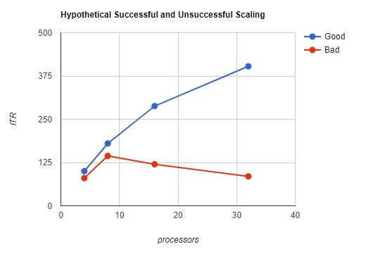
Of what use is the effective capability curve, then? The curve shows us the approximate shape of a successful scaling set. We are looking for gradual rolloff with no sharp inflection points. Figure 4 shows us hypothetical successful and unsuccessful runs.
| Figure 4. Hypothetical successful and unsuccessful scaling. |
|
| Notes: This hypothetical data shows the difference between a workload that scaled well and a workload that did not scale well. |
When a workload does not scale, we look to see what failed. To find the failure, we use MONWRITE data, z/VM Performance Toolkit reports, the CPU MF host counters, the lab-mode sampler, and anything else that might help. Common kinds of failures include use of algorithms that are too computationally complex, or excessive use of serialization, or inadvertent misuse of memory as relates to cache lines. When we find such failures, we make repairs as needed to meet the scaling goal.
The CAF curve and the effective capability curve tell us more than just what acceptable scaling looks like. At higher values of n, cn decreases to a point where it is clear there is a tradeoff to be made between the administrative convenience of having one large partition and the cost per unit of effective capability. For example, consider Table 3, which shows the capabilities of a number of different z14 deployments that exploit 80 processors in total.
| Table 3. Capabilities of various 80-processor z14 deployments. | |||
| Processors per partition | CAF Value | Number of partitions | Total capability |
| 80 | 0.554 | 1 | (1 x 80 x 0.554) = 44.32 |
| 40 | 0.622 | 2 | (2 x 40 x 0.622) = 49.76 |
| 20 | 0.693 | 4 | (4 x 20 x 0.693) = 55.44 |
| 10 | 0.802 | 8 | (8 x 10 x 0.802) = 64.16 |
| Notes: 3906-M05 s/n E4E67, 2019-03-30. | |||
A single large partition might be easier to maintain and administer, but the capability is less than the total capability of a number of smaller partitions. Customers considering large partitions will want to balance their need for low administrative cost against their need for efficient hardware exploitation. Further, though we don't like to think about them, the consequences of an outage of a single large partition as compared to those arising from the failure of only one of a number of smaller partitions also need to be considered.
Method
The studies presented here were all done with the Apache workload. A number of Linux guests running Application Workload Modeler (AWM) were configured to send HTTP transactions to a number of Linux guests running the Apache web server. All clients and all servers resided together in one single partition.
Two different arrangements of clients and servers were used.
-
The first was a monolithic arrangement where every client guest
directed HTTP transactions to every server guest. All client
guests and all server guests were coupled to a single
vswitch. To ramp up the workload we added client guests,
server guests, processors, and central memory.
Figure 5 illustrates the configuration.
Figure 5. Monolithic Apache workload. 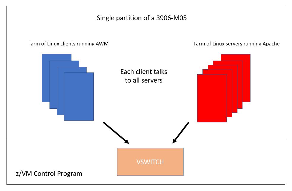
-
The next was an arrangement consisting of a number
of small groups
of client guests and server guests,
the members of each group
connected
to one another through a group-specific vswitch.
We called such an arrangement
a tiled arrangement.
Each tile consisted of some clients, some servers, and a vswitch.
All vswitches' uplink ports were
connected to
the same OSA chpid.
Each client guest sent HTTP
transactions to all the server guests on its tile.
To ramp up the
workload we added tiles, processors, and central memory.
There was no
inter-vswitch traffic during the steady-state portion of the
measurement.
Figure 6 illustrates the configuration.
Figure 6. Tiled Apache workload. 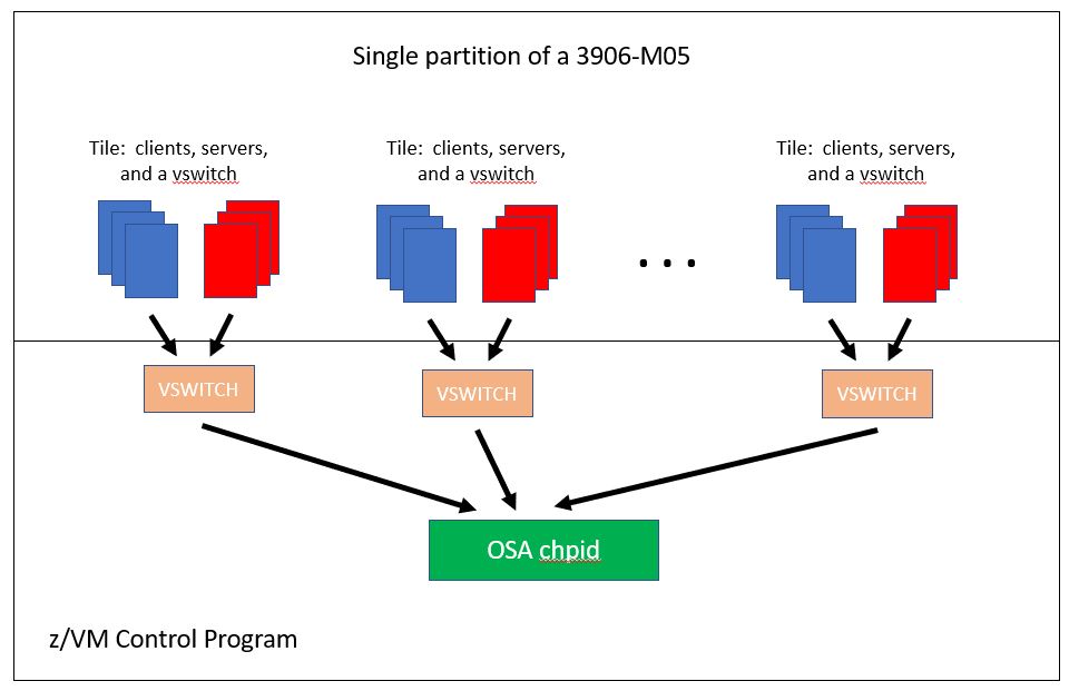
All measurements were collected on a 3906-M05. The partition was always dedicated, with all IFL processors. No other partitions were ever activated. The number of processors was varied according to the needs of the particular workload being run.
The z/VM CP load module used was a z/VM 7.1 module containing a pre-GA edition of the PTF. The pre-GA edition let us run beyond 80 logical processors. z/VM was always configured for non-SMT operation, and for vertical mode, and for UNPARKING LARGE.
All clients and all servers ran SLES 12 SP 3. In all cases the Linux guests were configured so they would not need to swap. Each guest had a virtual NIC coupled to a vswitch appropriate for the measurement.
Runs were done in both memory-rich and memory-constrained configurations.
-
For the memory-rich runs,
- All guests were virtual 1-ways with 1024 MB of guest real.
- The HTTP transactions sent were configured for what we call two small files. What this means is that every HTTP transaction sent from an AWM client to an Apache server was an HTTP GET of either one or the other of two small ballast files held in the Linux server's file system. In this way each server guest will retain the two ballast files in its Linux file cache.
- The numbers of clients, servers, and processors were chosen so that at the low end of the scaling set, FCX225 SYSSUMLG showed the average logical processor to be in the neighborhood of 90% busy. As we ramped up the configuration it was inevitable that the average logical processor would become more than 90% busy.
- Central memory was always set far above the needs of the workload.
-
For the memory-constrained runs,
- The client guests were all virtual 4-ways with 4096 MB of guest real. The server guests were all virtual 1-ways with 5 GB of guest real.
- HTTP transactions sent were configured for what we call 5,000 1-MB files. What this means is that every HTTP transaction sent from an AWM client to an Apache server was an HTTP GET of one out of 5,000 possible files, each file 1 MB in size. In this way, we drove paging I/O and also virtual I/O.
- FCX225 SYSSUMLG would not approach 90% busy because of limits in our paging subsystem.
- Central memory was chosen to create a paging rate consistent with the highest paging rates we could remember seeing in recent customer data.
- All runs were primed in the sense that the run was done twice back-to-back and the second run was the one from which measurements were collected.
The above configurations check scalability of basic z/VM CP functions such as scheduling, dispatching, interrupt handling, and handling of privileged operations. They also check scalability of intra-vswitch traffic. The memory-constrained configurations check scalability of virtual I/O, of memory management, and of paging I/O.
Results and Discussion
This section presents results for the memory-rich and memory-constrained evaluations.
Memory-Rich Workloads
Our first set of memory-rich runs was of monolithic Apache. For the base run we chose 9 clients, 36 servers, and 19 processors because this combination put us close to the target of running the average logical processor 90% busy. We used a layer-3 vswitch to connect the guests together. From that base run we ramped up, adding clients, servers, and processors, all in proportion. We ran this up to a 95-processor configuration. Table 4 shows the findings.
| Table 4. Monolithic Apache, layer-3 vswitch. | |||||
| Run ID | A9NZ524Y | AS2Z9140 | AS3Z9140 | AS4Z9140 | AS5Z9140 |
| Logical processors | 19 | 38 | 57 | 76 | 95 |
| Client guests | 9 | 18 | 27 | 36 | 40 |
| Server guests | 36 | 72 | 108 | 144 | 180 |
| ETR | 82817.32 | 155433.48 | 221439.86 | 265372.72 | 271351.24 |
| ITR | 86810.6 | 162587.3 | 226885.1 | 269962.1 | 271622.9 |
| Logical proc avg busy | 95.4 | 95.6 | 97.6 | 98.3 | 99.9 |
| ITRR wrt smallest run | 1.00 | 1.87 | 2.61 | 3.11 | 3.13 |
| Capability ratio | 1.00 | 1.80 | 2.53 | 3.21 | 3.87 |
| Notes: CEC model 3906-M05. Dedicated partition, storage-rich. z/VM 7.1 driver containing pre-GA PTF, vertical mode, non-SMT, UNPARKING LARGE. SLES 12 SP 3 with AWM and Apache. All guests 1-way and 1024 MB. Two small files. ITRR wrt smallest run is ITR of run divided by ITR of smallest run. Capability ratio is effective capability of the partition divided by effective capability of the smallest partition. | |||||
The ITRR (ITR ratio) values show that up to 57 processors, results exceeded the CAF prediction. But between 57 processors and 76 processors, ITR rolled off. We investigated this and found there was a code problem in the implementation of layer-3 vswitches. The code problem involved several aspects. First, associated with the layer-3 vswitch there was a list of control blocks that had to be searched repeatedly. The length of the list was equal to the number of VNICs coupled to the vswitch. Second, the control blocks on that list were being updated right after being found. Third, the control block's list pointers were in the same cache line as the control block field being updated. These factors conspired to slow down the run in the higher N-way configurations.
In studying the vswitch implementation we concluded we could work around the layer-3 problem if we were to move to a tiled arrangement, so that the number of VNICs coupled to any given layer-3 vswitch would be somewhat smaller. This led us to our second set of runs, illustrated in Table 5.
| Table 5. Tiled Apache 9x36, layer-3 vswitch. | ||||
| Run ID | AS1R2116 | AS2R2116 | AS3R2116 | AS4R2116 |
| Logical processors | 19 | 38 | 57 | 76 |
| Client guests | 9 | 18 | 27 | 36 |
| Server guests | 36 | 72 | 108 | 144 |
| Vswitches | 1 | 2 | 3 | 4 |
| ETR | 84330.31 | 162532.18 | 228187.21 | 294185.16 |
| ITR | 87570.4 | 166358.4 | 231427.2 | 298059.9 |
| Logical proc avg busy | 96.3 | 97.7 | 98.6 | 98.7 |
| ITRR wrt smallest run | 1.00 | 1.90 | 2.64 | 3.40 |
| Capability ratio | 1.00 | 1.80 | 2.53 | 3.21 |
| Notes: CEC model 3906-M05. Dedicated partition, storage-rich. z/VM 7.1 driver containing pre-GA PTF, vertical mode, non-SMT, UNPARKING LARGE. SLES 12 SP 3 with AWM and Apache. All guests 1-way and 1024 MB. Two small files. ITRR wrt smallest run is ITR of run divided by ITR of smallest run. Capability ratio is effective capability of the partition divided by effective capability of the smallest partition. | ||||
Seeing the 76-processor tiled run did not show the problem, we were confident our tiled approach was a successful workaround. Thus we did not bother to repeat the 95-processor run as a tiled one.
During our study of the layer-3 vswitch problem we learned some other important things. First, we found that layer-2 vswitches are implemented differently than layer-3 vswitches are. In particular, there are no linear searches in the layer-2 implementation. Second, we found that IBM recommends vswitch deployments that use a number of layer-2 vswitches, for reasons such as failover. Third, we found that surveys of customers suggest most customers are using layer-2. For these reasons we saw no need to repeat the monolithic set with a layer-2 vswitch. We proceeded to try a set of tiled layer-2 runs. This set is illustrated in Table 6.
| Table 6. Tiled Apache 9x36, layer-2 vswitch. | ||||
| Run ID | AS1Z216A | AS2Z216A | AS3Z216A | AS4Z216A |
| Logical processors | 19 | 38 | 57 | 76 |
| Client guests | 9 | 18 | 27 | 36 |
| Server guests | 36 | 72 | 108 | 144 |
| Vswitches | 1 | 2 | 3 | 4 |
| ETR | 86930.42 | 169233.84 | 241547.85 | 314145.88 |
| ITR | 89804.1 | 173217.9 | 245725.2 | 314145.9 |
| Logical proc avg busy | 96.8 | 97.7 | 98.3 | 100.0 |
| ITRR wrt smallest run | 1.00 | 1.93 | 2.74 | 3.50 |
| Capability ratio | 1.00 | 1.80 | 2.53 | 3.21 |
| Notes: CEC model 3906-M05. Dedicated partition, storage-rich. z/VM 7.1 driver containing pre-GA PTF, vertical mode, non-SMT, UNPARKING LARGE. SLES 12 SP 3 with AWM and Apache. All guests 1-way and 1024 MB. Two small files. ITRR wrt smallest run is ITR of run divided by ITR of smallest run. Capability ratio is effective capability of the partition divided by effective capability of the smallest partition. | ||||
Comparing the tiled layer-2 ITR values to the tiled layer-3 values showed that layer-2 vswitches are a better performer in this workload. Also, the layer-2 ITRR values exceeded the layer-3 ones. So not only is layer-2 a better performer in our workload, it also scales better.
Next we noticed the logical processor percent-busy values in the layer-2 set were higher than we would have liked. We remembered that IBM's reference workloads for processor scaling are run in a fashion that tries to hold percent-busy to about 90%. We tried adjusting the shape of the tile so as to bring percent-busy down a little. We changed the shape of the tile so that in the largest run we would be about 90% busy. This set is illustrated in Table 7.
| Table 7. Tiled Apache 7x36, layer-2 vswitch. | |||||
| Run ID | AS1Z216F | AS2Z216F | AS3Z216F | AS4Z216F | AS5Z216F |
| Logical processors | 19 | 38 | 57 | 76 | 95 |
| Client guests | 7 | 14 | 21 | 28 | 35 |
| Server guests | 36 | 72 | 108 | 144 | 180 |
| Vswitches | 1 | 2 | 3 | 4 | 5 |
| ETR | 66448.79 | 127483.36 | 176862.63 | 228846.15 | 292037.90 |
| ITR | 87088.8 | 156613.5 | 208564.4 | 260348.3 | 311009.5 |
| Logical proc avg busy | 76.3 | 81.4 | 84.8 | 87.9 | 93.9 |
| ITRR wrt smallest run | 1.00 | 1.80 | 2.39 | 2.99 | 3.57 |
| Capability ratio | 1.00 | 1.80 | 2.53 | 3.21 | 3.87 |
| Notes: CEC model 3906-M05. Dedicated partition, storage-rich. z/VM 7.1 driver containing pre-GA PTF, vertical mode, non-SMT, UNPARKING LARGE. SLES 12 SP 3 with AWM and Apache. All guests 1-way and 1024 MB. Two small files. ITRR wrt smallest run is ITR of run divided by ITR of smallest run. Capability ratio is effective capability of the partition divided by effective capability of the smallest partition. | |||||
In the above set we found ITRR did not do as well as the effective capability curve predicted. We feel this is because the ITR in the first run is optimistically high because percent-busy is too low. In other words, because we know the processor is more efficient at lower percents-busy, we also know a low percent-busy in the first run of the set will set the ITRR denominator too high for the subsequent larger runs and thereby depress the larger runs' ITRR values. Even so, we found the shape of the ITRR curve to be OK.
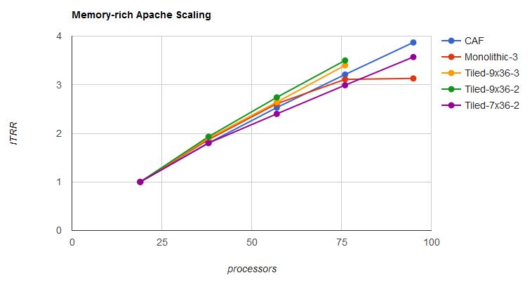
Figure 7 plots the effective capability curve and the ITRR curves for all the memory-rich runs. Up to the vicinity of 80 processors, all runs tracked at or near the effective capability curve.
| Figure 7. Scaling of various Apache memory-rich workloads. |
|
| Notes: Data from Table 4, Table 5, Table 6, and Table 7. |
Memory-Constrained Workload
Next we devised a tile and a partition configuration that together would produce the paging rate we wanted. This tile consisted of 5 clients, 60 servers, and one layer-2 vswitch, run in 16 processors and 256 GB of central memory. We then ramped this up by tiling, with the last size being 80 processors. Table 8 shows the results.
| Table 8. Tiled Apache DASD Paging, 5x60, layer-2 vswitch. | |||||
| Run ID | AP1Z604G | AP2Z604G | AP3Z604G | AP4Z604D | AP5Z604G |
| Logical processors | 16 | 32 | 48 | 64 | 80 |
| Central memory (GB) | 256 | 512 | 768 | 1024 | 1280 |
| Client guests | 5 | 10 | 15 | 20 | 25 |
| Server guests | 60 | 120 | 180 | 240 | 300 |
| Vswitches | 1 | 2 | 3 | 4 | 5 |
| ETR | 3295.34 | 2589.74 | 3239.92 | 4143.10 | 3745.58 |
| ITR | 5031.1 | 8778.8 | 12272.4 | 15873.9 | 18634.7 |
| Logical proc avg busy | 65.5 | 29.5 | 26.4 | 26.1 | 20.1 |
| Total guest busy | 658.6387 | 544.3393 | 703.7159 | 939.4967 | 858.4882 |
| Total chargeable CP busy | 296.5102 | 322.3837 | 476.6080 | 635.6118 | 630.1159 |
| Total non-chargeable CP busy | 92.7207 | 78.4516 | 85.5843 | 98.1747 | 117.7722 |
| Total partition busy | 1047.8696 | 945.1746 | 1265.9082 | 1673.2832 | 1606.3763 |
| System T/V | 1.59 | 1.74 | 1.80 | 1.78 | 1.87 |
| Guest busy/tx | 0.1999 | 0.2102 | 0.2172 | 0.2268 | 0.2292 |
| Chargeable CP busy/tx | 0.0900 | 0.1245 | 0.1471 | 0.1534 | 0.1682 |
| Non-chargeable CP busy/tx | 0.0281 | 0.0303 | 0.0264 | 0.0237 | 0.0314 |
| CP busy/tx | 0.1181 | 0.1548 | 0.1735 | 0.1771 | 0.1997 |
| CPUMF CPI | 3.004 | 3.105 | 3.226 | 3.447 | 3.429 |
| CPUMF EICPI | 1.183 | 1.155 | 1.129 | 1.135 | 1.146 |
| CPUMF EFCPI | 1.822 | 1.950 | 2.096 | 2.312 | 2.283 |
| CPUMF Inst/tx | 5528981.83 | 6138761.81 | 6319576.41 | 6113161.64 | 6525397.94 |
| z/VM paging rate | 211000.0 | 182000.0 | 184000.0 | 195000.0 | 201000.0 |
| Unparked processors | 16 | 32 | 48 | 64 | 80 |
| ITRR wrt smallest run | 1.000 | 1.745 | 2.439 | 3.155 | 3.704 |
| Capability ratio | 1.00 | 1.79 | 2.51 | 3.21 | 3.84 |
| Notes: CEC model 3906-M05. Dedicated partition, storage-constrained. z/VM 7.1 driver containing pre-GA PTF, vertical mode, non-SMT, UNPARKING LARGE, z/HPF paging. SLES 12 SP 3 with AWM and Apache. Client guests were 4-ways with 4096 MB of guest real. Server guests were 1-ways with 5 GB of guest real. 5,000 1-MB files. ITRR wrt smallest run is ITR of run divided by ITR of smallest run. Capability ratio is effective capability of the partition divided by effective capability of the smallest partition. | |||||
The above table shows a very interesting set of runs. First up is to look at why ETR did not scale. The reason is that the paging activity was too much for our paging DASD to handle. We used the z/VM Performance Toolkit DEVGROUP facility to look at the behavior of our paging volumes -- 224 3390-54 volumes spread over 16 LCUs, all in one storage server -- as we scaled up. From FCX108 DEVICE we found paging volume performance dropped rapidly as we scaled up. The rise in disconnect time suggests trouble in the storage server read cache. FCX176 CTLUNIT, not shown, corroborated this; in the smallest run we had a 96% read hit rate in the storage server, but in the largest run the read hit rate dropped to 58%.
(From FCX108 DEVICE)

          <-- Device Descr. -->  Mdisk Pa- <-Rate/s-> <------- Time (msec) -------> Req. <Percent>
Run       Addr Type   Label/ID   Links ths  I/O Avoid Pend Disc Conn Serv Resp CUWt Qued Busy READ

AP1Z604G  PAGING                  ....  ..  180    .0 .147 .479 .229 .855 1.50 .000  .12   15   97
AP2Z604G  PAGING                  ....  .. 89.4    .0 .156 2.77 .271 3.19 6.46 .000  .29   29   93
AP3Z604G  PAGING                  ....  .. 48.0    .0 .208 7.39 .418 8.02 18.0 .000  .47   38   86
AP4Z604D  PAGING                  ....  .. 43.4    .0 .240 9.58 .483 10.3 25.2 .000  .66   45   84
AP5Z604G  PAGING                  ....  .. 45.5    .0 .241 10.5 .480 11.2 30.8 .000  .89   51   84
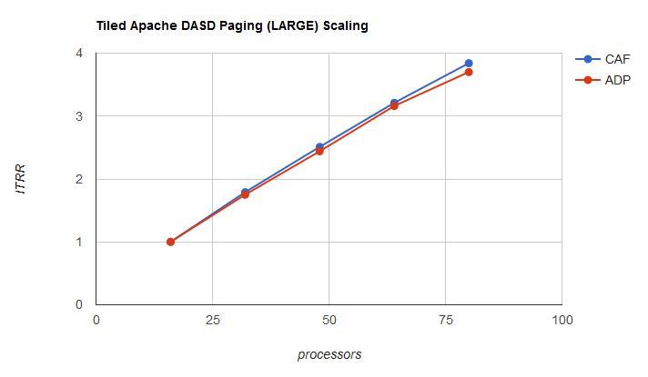
Next up is to look at how the runs' ITRR curve tracks the effective capability curve. Figure 8 shows the two curves.
| Figure 8. Scaling of Apache DASD Paging (ADP) memory-constrained workload. |
|
| Notes: Data from Table 8. |
The runs' ITRR curve tracks not too far below the effective capability curve. However, in looking at Table 8 we noticed logical processor average busy decreased as partition size increased. This relationship means the ITR values in large partitions might be optimistic compared to the ITR produced in the base run, and so the scaling picture presented in the graph might be optimistic.
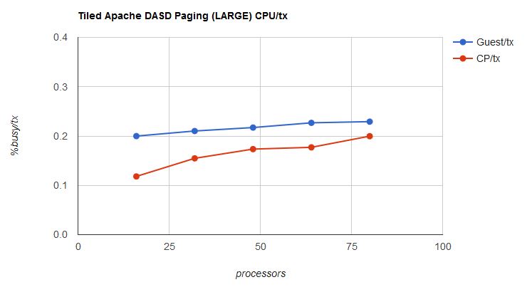
We also noticed that percent-busy isn't all that high in these workloads, and further, system T/V is climbing as the partition gets larger. When we see these two situations together, our thought is usually that CP is struggling to deal with the situation that there isn't all that much CP work to do compared to the number of processors trying to do it. To check this out we calculated and plotted guest CPU-busy per transaction and CP CPU-busy per transaction as a function of run size. Figure 9 shows the two curves.
| Figure 9. Tiled Apache DASD Paging, guest busy/tx and CP busy/tx. |
|
| Notes: Data from Table 8. |
The graph shows that guest/tx and CP/tx track pretty well to each other. The largest run does show an uptick in CP/tx. This suggests CP is feeling the effect of the wide partition.
At the high end we noticed we were running the average logical processor around 20% busy and all 80 logical processors were engaged. Knowing PR/SM was having to dispatch all those logical processors on physical processors, and seeing that the partition wasn't terribly busy, we decided to try UNPARKING SMALL to see whether we could get comparable results while disposing of apparently excess logical processors. Table 9 shows the result.
| Table 9. Tiled Apache DASD Paging, 5x60, layer-2 vswitch, UNPARKING SMALL. | |||||
| Run ID | AP1Z604F | AP2Z604D | AP3Z604D | AP4Z604H | AP5Z604D |
| Logical processors | 16 | 32 | 48 | 64 | 80 |
| Central memory (GB) | 256 | 512 | 768 | 1024 | 1280 |
| Client guests | 5 | 10 | 15 | 20 | 25 |
| Server guests | 60 | 120 | 180 | 240 | 300 |
| Vswitches | 1 | 2 | 3 | 4 | 5 |
| ETR | 3184.44 | 2547.23 | 3133.38 | 2988.47 | 3417.83 |
| ITR | 4921.9 | 9262.7 | 12737.3 | 15812.0 | 18987.9 |
| Logical proc avg busy | 64.7 | 27.5 | 24.6 | 18.9 | 18.0 |
| Total guest busy | 651.4086 | 563.3618 | 779.8798 | 806.4922 | 961.4873 |
| Total chargeable CP busy | 288.0558 | 252.9631 | 342.3203 | 338.2278 | 409.1662 |
| Total non-chargeable CP busy | 95.7314 | 62.5358 | 59.5531 | 66.7100 | 69.4481 |
| Total partition busy | 1035.1958 | 878.8607 | 1181.7532 | 1211.4300 | 1440.1016 |
| System T/V | 1.59 | 1.56 | 1.52 | 1.50 | 1.50 |
| Guest busy/tx | 0.2046 | 0.2212 | 0.2489 | 0.2699 | 0.2813 |
| Chargeable CP busy/tx | 0.0905 | 0.0993 | 0.1092 | 0.1132 | 0.1197 |
| Non-chargeable CP busy/tx | 0.0301 | 0.0246 | 0.0190 | 0.0223 | 0.0203 |
| CP busy/tx | 0.1205 | 0.1239 | 0.1283 | 0.1355 | 0.1400 |
| CPUMF CPI | 3.066 | 3.062 | 3.306 | 3.601 | 3.510 |
| CPUMF EICPI | 1.196 | 1.169 | 1.133 | 1.181 | 1.135 |
| CPUMF EFCPI | 1.870 | 1.893 | 2.173 | 2.420 | 2.375 |
| CPUMF Inst/tx | 5535766.41 | 5876959.68 | 5947287.59 | 5868276.74 | 6257968.36 |
| z/VM paging rate | 217000.0 | 180000.0 | 186000.0 | 219000.0 | 198000.0 |
| Unparked processors | 13.4 | 12.0 | 15.5 | 15.6 | 18.5 |
| ITRR wrt smallest run | 1.000 | 1.882 | 2.588 | 3.213 | 3.858 |
| Capability ratio | 1.00 | 1.79 | 2.51 | 3.21 | 3.84 |
| Notes: CEC model 3906-M05. Dedicated partition, storage-constrained. z/VM 7.1 driver containing pre-GA PTF, vertical mode, non-SMT, UNPARKING SMALL, z/HPF paging. SLES 12 SP 3 with AWM and Apache. Client guests were 4-ways with 4096 MB of guest real. Server guests were 1-ways with 5 GB of guest real. 5,000 1-MB files. ITRR wrt smallest run is ITR of run divided by ITR of smallest run. Capability ratio is effective capability of the partition divided by effective capability of the smallest partition. | |||||
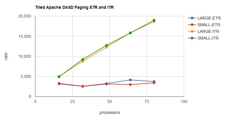
Figure 10 shows ETR and ITR of the UNPARKING LARGE set and of the UNPARKING SMALL set.
| Figure 10. Tiled Apache DASD Paging, effect of UNPARKING SMALL on ETR and ITR. |
|
| Notes: Data from Table 8 and Table 9. |
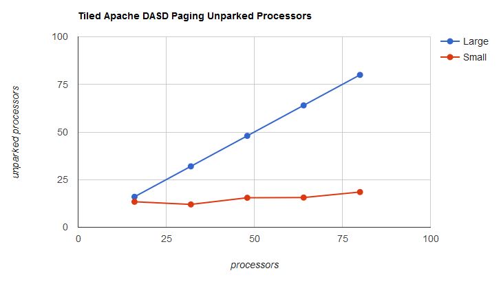
Aside from one deviation, the performance experience with UNPARKING SMALL was not much different from the experience with UNPARKING LARGE. The big difference is in the dispatch burden the two sets exerted upon PR/SM. In the UNPARKING LARGE cases, PR/SM had to juggle all of the partition's logical processors. In the UNPARKING SMALL cases, PR/SM had to dispatch only the unparked logical processors. In other words, parking unneeded logical processors freed up physical cores for PR/SM to use for other purposes, such as to run other partitions. In the largest UNPARKING SMALL run, z/VM gave about 60 physical cores back to PR/SM with no appreciable performance impact. Figure 11 shows the difference.
| Figure 11. Tiled Apache DASD Paging, number of unparked processors. |
|
| Notes: Data from Table 8 and Table 9. |
There are some other effects of UNPARKING SMALL worth exploring. One effect worth looking at is average logical processor percent busy on the unparked processors. Table 9 is a little misleading in that it suggests the unparked logical processors were in the neighborhood of 25% busy. This isn't true. Table 10 shows average busy per average unparked processor. UNPARKING SMALL squeezes the work into the smallest number of logical processors it seems would suffice to run the workload.
| Table 10. Tiled Apache DASD Paging, percent-busy of average unparked processor. | |||||
| Logical processors | 16 | 32 | 48 | 64 | 80 |
| LARGE Run ID | AP1Z604G | AP2Z604G | AP3Z604G | AP4Z604D | AP5Z604G |
| Avg number of unparked processors | 16 | 32 | 48 | 64 | 80 |
| %Busy of avg unparked processor | 65.5 | 29.5 | 26.4 | 26.1 | 20.1 |
| SMALL Run ID | AP1Z604F | AP2Z604D | AP3Z604D | AP4Z604H | AP5Z604D |
| Avg number of unparked processors | 13.4 | 12.0 | 15.5 | 15.6 | 18.5 |
| %Busy of avg unparked processor | 77.2 | 73.2 | 76.3 | 77.6 | 77.8 |
| Notes: CEC model 3906-M05. Dedicated partition, storage-constrained. z/VM 7.1 driver containing pre-GA PTF, vertical mode, non-SMT. SLES 12 SP 3 with AWM and Apache. Client guests were 4-ways with 4096 MB of guest real. Server guests were 1-ways with 5 GB of guest real. 5,000 1-MB files. | |||||
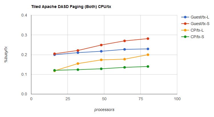
Another effect worth looking at is the change in CPU/tx. Figure 12 shows how CPU/tx in guest and CP changed with unparking model. In UNPARKING SMALL, CP had to deal with far less parallelism and so we could expect its CPU/tx to decrease, because it would spend less time spinning on locks. FCX326 LOCKACT, not shown, corroborated this. At the same time, the guests, squeezed into fewer, much busier logical processors, would experience far more cramped quarters and so we could expect their CPU/tx to rise from cache effects. In our particular case, the increase in guest CPU/tx was just about balanced out by decrease in CP CPU/tx. This is why the ITR curves of the LARGE and SMALL sets are nearly the same.
| Figure 12. Tiled Apache DASD Paging, effect of unparking model on CPU/tx. |
|
| Notes: Data from Table 8 and Table 9. |
Another effect of UNPARKING SMALL is change in dispatch latency. From queueing theory we know that when the service points become more busy, those waiting in line wait longer to be served. z/VM tracks the wait time dispatchable virtual CPUs spend waiting to be dispatched. The data comes out in D4 R3 MRUSEACT records. z/VM Performance Toolkit does not tabulate the data but IBM has a tool that does so. Table 11 illustrates what the tool found for the UNPARKING LARGE set and for the UNPARKING SMALL set. We can see that in the UNPARKING SMALL set, dispatchable virtual CPUs spent more time waiting for dispatch. However, transaction response time was not affected. This means transaction response time was dominated by some other factor, likely the intense paging.
| Table 11. Tiled Apache DASD Paging, 5x60, layer-2 vswitch. | |||||
| Logical processors | 16 | 32 | 48 | 64 | 80 |
| LARGE Run ID | AP1Z604G | AP2Z604G | AP3Z604G | AP4Z604D | AP5Z604G |
| Unparked processors | 16 | 32 | 48 | 64 | 80 |
| Mean dispatch wait, clients (μsec) | 0.36 | 0.60 | 0.66 | 0.90 | 0.73 |
| Mean dispatch wait, servers (μsec) | 6.50 | 2.20 | 2.43 | 3.26 | 1.76 |
| Transaction resp time, msec | 0.10247 | 0.22646 | 0.28252 | 0.35268 | 0.44371 |
| SMALL Run ID | AP1Z604F | AP2Z604D | AP3Z604D | AP4Z604H | AP5Z604D |
| Unparked processors | 13.4 | 12.0 | 15.5 | 15.6 | 18.5 |
| Mean dispatch wait, clients (μsec) | 1.23 | 9.58 | 11.78 | 17.89 | 16.22 |
| Mean dispatch wait, servers (μsec) | 23.78 | 87.28 | 145.23 | 208.51 | 257.17 |
| Transaction response time, msec | 0.09351 | 0.22755 | 0.27875 | 0.40280 | 0.40499 |
| Notes: CEC model 3906-M05. Dedicated partition, storage-constrained. z/VM 7.1 driver containing pre-GA PTF, vertical mode, non-SMT. SLES 12 SP 3 with AWM and Apache. Client guests were 4-ways with 4096 MB of guest real. Server guests were 1-ways with 5 GB of guest real. 5,000 1-MB files. | |||||
Summary
Eighty Logical Processors provides support, on the z14, for up to 80 logical processors in a partition. To check scalability, we ran memory-rich and memory-constrained workloads. In the workloads we ran, the system usually scaled correctly. The notable exception was when we tried to put all clients and all servers in a large partition onto a single layer-3 vswitch. The workaround there was to change to a tiled configuration.
Our memory-constrained workload had modest CPU utilization in a very large partition and so it gave us an opportunity to exercise UNPARKING SMALL. Using UNPARKING SMALL caused z/VM to release physical cores to PR/SM, thereby giving PR/SM the opportunity to use those cores for other purposes. However, because CPU utilization on the unparked processors was so much larger than it was in the UNPARKING LARGE case, virtual CPU dispatch wait time increased. For our workload the increase was of no consequence, but for other workloads the increase might have consequences, such as affecting transaction response time. Customers pondering UNPARKING SMALL will want to collect measures of application success, such as ETR, transaction response time, and conformance to SLAs, before and after, so they can find the correct balance for their environments.